figure below shows the scope blocks

- Scope, Floating Scope, Signal Viewer Scope
Display signals generated during a simulation
The Scope block displays its input with respect to simulation time. The Scope block can have multiple axes (one per port); all axes have a common time range with independent y-axes. The Scope allows you to adjust the amount of time and the range of input values displayed. You can move and resize the Scope window and you can modify the Scope's parameter values during the simulation.
When you start a simulation, Simulink does not open Scope windows, although it does write data to connected Scopes. As a result, if you open a Scope after a simulation, the Scope's input signal or signals will be displayed.
If the signal is continuous, the Scope produces a point-to-point plot. If the signal is discrete, the Scope produces a stair-step plot.
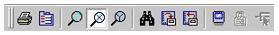
The Scope provides toolbar buttons that enable you to zoom in on displayed data, display all the data input to the Scope, preserve axis settings from one simulation to the next, limit data displayed, and save data to the workspace. The toolbar buttons are labeled in this figure, which shows the Scope window as it appears when you open a Scope block.
Note: Do not use Scope blocks inside library blocks that you create. Instead, provide the library blocks with output ports to which scopes can be connected to display internal data.
- Displaying Vector Signals
When displaying a vector or matrix signal, the Scope assigns colors to each signal element in this order: yellow, magenta, cyan, red, green, and dark blue. When more than six signals are displayed, the Scope cycles through the colors in the order listed.
You set y-limits by right-clicking an axis and choosing Axes Properties. The following dialog box appears.

Enter the maximum value for the y-axis.
Enter the title of the plot. You can include a signal label in the title by typing % as part of the title string (% is replaced by the signal label).
This figure shows the Scope block displaying the output of the vdp model. The simulation was run for 40 seconds. Note that this scope shows the final 20 seconds of the simulation. The Time offset field displays the time corresponding to 0 on the horizontal axis. Thus, you have to add the offset to the fixed time range values on the x-axis to get the actual time.

- Autoscaling the Scope Axes
This figure shows the same output after you click the Autoscale toolbar button, which automatically scales both axes to display all stored simulation data. In this case, the y-axis was not scaled because it was already set to the appropriate limits.

If you click the Autoscale button while the simulation is running, the axes are autoscaled based on the data displayed on the current screen, and the autoscale limits are saved as the defaults. This enables you to use the same limits for another simulation.
Note:Simulink does not buffer the data that it displays on a floating Scope. It can therefore scale the contents of a floating Scope only when data is being displayed, i.e., when a simulation is running. When a simulation is not running, Simulink disables (grays) the Zoom button on the toolbar of a floating Scope to indicate that it cannot scale its contents.
You can zoom in on data in both the x and y directions at the same time, or in either direction separately. The zoom feature is not active while the simulation is running.
To zoom in on data in both directions at the same time, make sure you select the leftmost Zoom toolbar button. Then, define the zoom region using a bounding box. When you release the mouse button, the Scope displays the data in that area. You can also click a point in the area you want to zoom in on.
If the scope has multiple y-axes, and you zoom in on one set of x-y axes, the x-limits on all sets of x-y axes are changed so that they match, because all x-y axes must share the same time base (x-axis).
This figure shows a region of the displayed data enclosed within a bounding box.

This figure shows the zoomed region, which appears after you release the mouse button.

To zoom in on data in just the x direction, click the middle Zoom toolbar button. Define the zoom region by positioning the pointer at one end of the region, pressing and holding down the mouse button, then moving the pointer to the other end of the region. This figure shows the Scope after you define the zoom region, but before you release the mouse button.

When you release the mouse button, the Scope displays the magnified region. You can also click a point in the area you want to zoom in on.
Zooming in the y direction works the same way except that you click the rightmost Zoom toolbar button before defining the zoom region. Again, you can also click a point in the area you want to zoom in on.
Note: Simulink does not buffer the data that it displays on a floating scope. It therefore cannot zoom the contents of a floating scope. To indicate this, Simulink disables (grays) the Zoom button on the toolbar of a floating scope.
The Save axes settings toolbar button enables you to store the current x- and y-axis settings so you can apply them to the next simulation.

You might want to do this after zooming in on a region of the displayed data so you can see the same region in another simulation. The time range is inferred from the current x-axis limits.
The Scope Parameters dialog box lets you change axis limits, set the number of axes, time range, tick labels, sampling parameters, and saving options. To display the dialog, select the Parameters button on the toolbar of the Scope block's display.

or by double-clicking on the Scope viewer's display. The appearance of the dialog box depends on whether the scope is a Scope block or a Scope viewer created by the Signal and Scope Manager. If the scope is a Scope block, this dialog appears.

The dialog box has two panes: General and Data history. See the next topic for information on the General parameters pane. See Data History Parameters Pane for information on the Data History parameters pane.
If the scope is a Scope viewer, this dialog box appears.

You can set the axis parameters, time range, and tick labels in the General pane.
Set the number of y-axes in this data field. With the exception of the floating scope, there is no limit to the number of axes the Scope block can contain. All axes share the same time base (x-axis), but have independent y-axes. Note that the number of axes is equal to the number of input ports.
Change the x-axis limits by entering a number or auto in the Time range field. Entering a number of seconds causes each screen to display the amount of data that corresponds to that number of seconds. Enter auto to set the x-axis to the duration of the simulation. Do not enter variable names in these fields.
Specifies whether to label axes tics. The options are:
- all
- Label tics on the outside of all axes
- inside
- Place tic labels inside all axes (available only on scope viewers)
- bottom-axis only
- Place tic labels outside the bottom (or only) axes
- none
Do not label tics (available only on Scope blocks)
Note The next three options appear only for the dialog box for a Scope viewer
When this option is selected, the scope continuously scrolls the displayed signals to the left so as to keep as much of them in view as will fit on the screen at any one time. When this option is not selected, the scope draws a screenful of data from left to right until the screen is full, erases the screen and draws the next screenful of data, and so on, until the end of simulation time. Note that the effects of this option are discernible only when drawing is slow, for example, when the model is very large or has a very small step size.
Displays a marker at each data point on the scope viewer screen

Displays a legend on the scope that indicates the line style used to display each signal

This option appears only on the General parameters pane for the Scope block.
Selecting this option turns a Scope block into a floating scope. A floating scope is a Scope block that can display the signals carried on one or more lines. You can create a Floating Scope block in a model either by copying a Scope block from the Simulink Sinks library into a model and selecting this option or, more simply, by copying the Floating Scope block from the Sinks library into the model window. The Floating Scope block has the Floating scope parameter selected by default.
To use a floating scope during a simulation, first open the scope. To display the signals carried on a line, select the line. Hold down the Shift key while clicking another line to select multiple lines. It might be necessary to click the Autoscale data button on the floating scope's toolbar to find the signal and adjust the axes to the signal values. Or you can use the floating scope's Signal Selector (see The Signal Selector in the online Simulink documentation) to select signals for display. To display a floating scope's Signal Selector, first start the simulation of your model with the floating scope open. Then right-click your mouse in the floating scope and select Signal Selection from the pop-up menu that appears.
You can have more than one floating scope in a model, but only one set of axes in one scope can be active at a given time. Active floating scopes show the active axes by making them blue. Selecting or deselecting lines affects the active floating scope only. Other floating scopes continue to display the signals that you selected when they were active. In other words, inactive floating scopes are locked, in that their signal displays cannot change.
To specify display of a signal on one of the axes of a multiaxis floating scope, click the axis. Simulink draws a blue border around the axis.

Then click the signal you want to display in the block diagram or the Signal Selector. When you run the model, the selected signal appears in the selected axis.

If you plan to use a floating scope during a simulation, you should disable signal storage reuse. See "Signal storage reuse" in "The Optimization Pane" for more information.
Sampling
To specify a decimation factor, enter a number in the data field to the right of the Decimation choice. To display data at a sampling interval, select the Sample time choice and enter a number in the data field.
- Data History Parameters Pane
The Data History parameters pane appears only on the Parameters dialog box for the Scope block. The pane appears as follows:

This pane lets you control the amount of data that the Scope stores and displays. You can also choose to save data to the workspace in this pane. You apply the current parameters and options by clicking the Apply or OK button. The values that appear in these fields are the values that are used in the next simulation.
- Limit data points to last
You can limit the number of data points saved to the workspace by selecting the Limit data points to last check box and entering a value in its data field. The Scope relies on its data history for zooming and autoscaling operations. If the number of data points is limited to 1,000 and the simulation generates 2,000 data points, only the last 1,000 are available for regenerating the display.
You can automatically save the data collected by the Scope at the end of the simulation by selecting the Save data to workspace check box. If you select this option, the Variable name and Format fields become active.
Enter a variable name in the Variable name field. The specified name must be unique among all data logging variables being used in the model. Other data logging variables are defined on other Scope blocks, To Workspace blocks, and simulation return variables such as time, states, and outputs. Being able to save Scope data to the workspace means that it is not necessary to send the same data stream to both a Scope block and a To Workspace block.
Data can be saved in one of three formats: Array, Structure, or Structure with time. Use Array only for a Scope with one set of axes. For Scopes with more than one set of axes, use Structure if you do not want to store time data and use Structure with time if you want to store time data.
Performance Parameters Pane
The Performance parameters pane appears only on the Parameters dialog box for the Scope viewer. The pane appears as follows.

This pane lets you control how frequently Simulink refreshes the Scope viewer. Reducing the refresh rate can speed up the simulation in some cases. The pane contains the following controls.
This list control lets you select the units in which the refresh period is expressed. Options are either seconds or frames where a frame is the width of the scope's screen in seconds, i.e., it equals the value of the scope's Time range parameter.
Drag the slider button to the right to increase the refresh period and hence decrease the refresh rate.
Click the button to freeze (stop refreshing) or unfreeze the Scope viewer.
The History parameters pane appears only on the Parameters dialog box for the Scope viewer.

This pane lets you control the amount of data that the Scope viewer stores and displays. You can also choose to save data to the workspace in this pane. You apply the current parameters and options by clicking the Apply or OK button. The values that appear in these fields are the values that are used in the next simulation.
- Limit data points to last
You can limit the number of data points saved to the workspace by selecting the Limit data points to last check box and entering a value in its data field. The Scope relies on its data history for zooming and autoscaling operations. If the number of data points is limited to 1,000 and the simulation generates 2,000 data points, only the last 1,000 are available for regenerating the display.
Check this option to save data displayed on the scope viewer at the end of the simulation. Simulink saves the data in the Simulink.ModelDataLogs object used to log data for the model (see Logging Signals for more information). For this option to take effect, you must also enable signal logging for the model as a whole, i.e., you must check the Signal logging option on the Data Import/Export pane of the model's Configuration Parameters dialog box.
Variable name
Specifies the name under which to store the viewer's data in the model's Simulink.ModelDataLogs object. The name must be different from the log names specified by other signal viewers or for other signals, subsystems, or model references logged in the model's Simulink.ModelDataLogs object.
- Printing the Contents of a Scope Window
To print the contents of a Scope window, open the Print dialog box by clicking the Print icon, the leftmost icon on the Scope toolbar
The Scope block accepts real signals of any data type supported by Simulink, including fixed-point data types. The Scope block accepts homogeneous vectors.
For a discussion on the data types supported by Simulink, see Data Types Supported by Simulink in the Simulink documentation.
Characteristics

Thank you


